1. Brownian Motion
Markov Processes
The future only depends on the present state of the system and not the past\[ P(X_{t+1}=x | X_{t}=x_n, X_{t-1}=x_{t-1} , ... , X_{1}=x_1 ) = P(X_{t+1}=x | X_{t}=x_t ) \]
For discrete systems a map \[X_{t+1} = F(X_t,X_{t-1},...,t,\xi_t) \] simplifies to \[ X_{t+1} = F(t_t,\xi_t) \]
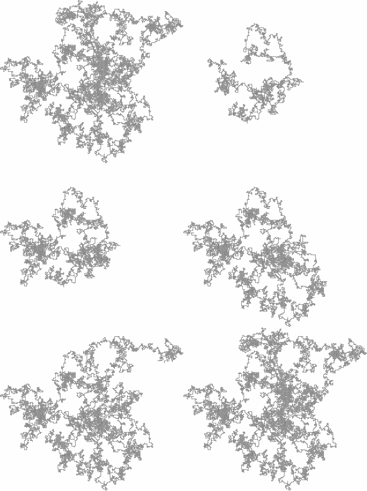
The Random Walk
Discrete process \[X_{t+1}=X_{t}+\xi_{t}\]
In one or more dimensions
 source:wikipedia.org
Randomness and Uncertainty
- Random variables in discrete or continuous time\[\xi_t \mbox{ or } \xi(t)\]
- Independence:\[ P(\xi(t_1)=a_1 \land \xi(t_2)=a_2) = P(\xi(t_1)=a_1) \cdot P(\xi(t_2)=a_2) \]
- Random variables and stochastic processes X(t) have a Probability Density Function (PDF) \[\rho(X) \mbox{ with } \int \rho(X) \mathrm{d}X = 1 \]
- For an ensemble of processes, values of all realizations at one point in time are distributed according to the PDF
- With the ensemble average, observables like the mean and variance are given as \[ \langle X(t) \rangle = \int X\rho(X) \mathrm{d}X = \mu \;\; \mbox{ and } \;\; \langle (X-\mu)^2 \rangle = \int (X-\mu)^2\rho(X) \mathrm{d}X = \sigma \]
- In many cases, a natural choice is the Gaussian normal distribution with zero mean \[ \rho(\xi) = \frac{1}{2\pi \sigma^2} e^-\frac{\xi^2}{2\sigma^2} \]
The Wiener Process
- Continuous version of the random walk
- Defined by \[ W_0=0 \] \[ \mbox{For all times } t_n>t_{n-1}>...>t_4>t_3>t_2>t_1: W_{t_2}-W_{t_1} \mbox{, } W_{t_4}-W_{t_3} \mbox{,... and } W_{t_n}-W_{t_{n-1}} \mbox{ are independent} \] \[ W_{t_n}-W_{t_{n-1}} \mbox{ all follow a Gaussian normal distribution}\]
- Self Similarity
 source:wikipedia.org
The Mean Squared Displacement (MSD)
A measure for fluctuations in a stochastic process \[ \langle (x(t)-x(0))^2 \rangle = \langle \int_0^t \dot{x}(s) \mathrm{d}s \int_0^t \dot{x}(q) \mathrm{d}q \rangle = \langle 2 \int_{0}^{t} \mathrm{d}t_1 \int_{t_1}^t \mathrm{d}t_2 \dot{x}(t_1) \dot{x}(t_2) \rangle = 2 \int_{0}^{t} \mathrm{d}t_1 \int_{t_1}^t \mathrm{d}t_2 \langle \dot{x}(t_1) \dot{x}(t_2) \rangle \]
with
\[ x(t)-x(0) = \int_0^t \dot{x}(s) \mathrm{d}s \]Wiener Process:
\[ \langle \dot{x}(t_1) \dot{x}(t_2) \rangle \approx D\delta(t_1-t_2) \] \[ \langle (x(t)-x(0))^2 \rangle = 2 D t \]The MSD scales linearly
Stochastic Differential equations
- Dynamics in continuous time
- Dynamics can be described via \[\dot{x}=F(x,t,\xi)\]
- For example: \[ dx = a dt + \sqrt{b} dW \]
- Solutions of Stochastic differential equations: the Ito-Integral \[\int_0^t C(x) \mathrm{d}W_t = \lim_{N\rightarrow \infty} \sum_{t_i\in [0,1]}^{N} C(x_{t_i}) (W_{t_{i+1}}-W_{t_{i}})\]
The Fokker-Planck equation
\[ \frac{\partial}{\partial t} \rho(x,t) = -\frac{\partial}{\partial x} a(x) \rho(x,t) + \frac{1}{2} \frac{\partial^2}{\partial x^2} b(x) \rho(x,t) \]- Drift term a(x), diffusion term b(x), both can be related to the Langevin equation
- Example: the Wiener Process \[ \frac{\partial \rho(x,t)}{\partial t} = \frac{1}{2} \frac{\partial^2 \rho(x,t)}{\partial x^2} \] Solved by \[ \rho(x,t) = \frac{1}{\sqrt{2\pi t}} e^{-x^2/(2t)} \]
Brownian Motion
Physical phenomenon, that was described by Robert Brown 1827 after seeing pollen in water under a microscope
\[\mbox{with viscosity } \eta, \mbox{ molecule radius } a, \mbox{ Bolztmann constant } k, \mbox{ temperature } T, \mbox{ and mass } m \]Derivation from Langevin equation
\[m\ddot{x} = - 6\pi \eta a \dot{x} + \xi\] \[\frac{m}{2}\frac{\mathrm{d}^2}{\mathrm{d}t^2} x^2 - mv^2 = -3\pi\eta a \frac{\mathrm{d}}{\mathrm{d}t} x^2 + \xi x\] \[\frac{m}{2}\frac{\mathrm{d}^2}{\mathrm{d}t^2} \langle x^2\rangle +3\pi\eta a \frac{\mathrm{d}}{\mathrm{d}t} \langle x^2\rangle = kT \mbox{ with } \langle\frac{1}{2}mv^2\rangle = \frac{1}{2}kT\] \[\langle x^2 \rangle = \frac{2kT}{m} \tau^2 \left[ \frac{t}{\tau} - (1-e^{-t/\tau}) \right] \mbox{ with } \tau=\frac{m}{6\pi\eta a}\] \[\langle x^2 \rangle \stackrel{t\gg \tau}{=} 2Dt \mbox{ with } D=\frac{kT}{ 6\pi\eta a}\]Perspective
- Random walk, Wiener Process, and Brownian Motion are not the same process!
- However, data has a finite resolution
- So, from the perspective of data analysis there is no difference
- the MSD is the same
- the Distribution as well, also see The Central Limit Theorem