4. Non-Gaussian Prozesses
The Gaussian Normal Distribution
\[\rho(x)=\frac{1}{\sqrt{2\pi} \sigma} e^-\frac{(x-\mu)^2}{2\sigma^2}\]Sum of two Random Numbers
- Look at histogram \[ P(x+y=z) = \sum_{x\leq z} P(x) P(y=z-x) \]
- Continuous limit: convolution \[ \rho_{x+y}(z) = \int \rho_x(x)\rho_y(z-x)\mathrm{d}x \]
Sum of two Gaussian Random Numbers
\[ \rho_{x+y}(z) = \int_{-\infty}^\infty \rho_x(x) \rho_y(z-x) \mathrm{d}x = \int_{-\infty}^\infty \frac{1}{\sqrt{2\pi} \sigma_x} e^-\frac{(x-\mu_x)^2}{2\sigma_x^2} \frac{1}{\sqrt{2\pi} \sigma_y} e^-\frac{(z-x-\mu_y)^2}{2\sigma_y^2} \mathrm{d}x \] \[ ... = \int_{-\infty}^\infty \frac{1}{\sqrt{2\pi}\sqrt{2\pi}\sigma_x\sigma_y} e^{-\frac{x^2(\sigma_x^2\sigma_y^2)-2x(\sigma_x^2(z-\mu_y)+\sigma_y^2\mu_x) + \sigma_x^2(z^2+\mu_y^2-2z\mu_y)+\sigma_y^2\mu_x^2}{2\sigma_y^2\sigma_x^2}} \mathrm{d}x \] \[ \mbox{with } \sigma_{x+y}^2=\sigma_x^2 + \sigma_y^2 \; \; \mbox{ and } \mu_{x+y}=\mu_x + \mu_y\] \[ ... = \frac{1}{\sqrt{2\pi}\sigma_{x+y}} e^{-\frac{(z-\mu_{x+y})^2}{2\sigma_{x+y}^2}} \int_{-\infty}^\infty \frac{1}{\sqrt{2\pi}\frac{\sigma_x\sigma_y}{\sigma_{x+y}}} e^{-\frac{\left(x-\frac{\sigma_x^2(z-\mu_y)+\sigma_y^2\mu_x}{\sigma_{x+y}^2}\right)^2}{2\left(\frac{\sigma_x\sigma_y}{\sigma_{x+y}}\right)^2}} \mathrm{d}x = \frac{1}{\sqrt{2\pi}\sigma_{x+y}} e^{-\frac{(z-\mu_{x+y})^2}{2\sigma_{x+y}^2}} \]Moments
A probability distribution can be defined by its moments
\[M_i = \int x^i \rho(x) \mathrm{d}x\]In the case of the Gaussian distribution, the moments are
\[M_1 = \frac{1}{2\pi \sigma^2} \int x e^-\frac{(x-\mu)^2}{2\sigma^2} \mathrm{d}x = \mu. \mbox{ In the following we set }\mu=0,\] i.e. we calculate the central moments \[M_2 = \frac{1}{2\pi \sigma^2} \int x^2 e^-\frac{x^2}{2\sigma^2} \mathrm{d}x = \sigma^2, \mbox{ } M_3 = \frac{1}{2\pi \sigma^2} \int x^3 e^-\frac{x^2}{2\sigma^2} \mathrm{d}x = 0, and\] \[M_4 = \frac{1}{2\pi \sigma^2} \int x^4 e^-\frac{x^2}{2\sigma^2} \mathrm{d}x = 3\sigma^4, \mbox{ i.e. } M_{i} = \left\lbrace\begin{array}{2} 0 & \mbox{i odd}\\ (i-1)!! \sigma^i & \mbox{i even}\end{array}\right.\]- The distribution is characterized by two parameters: mean and variance
The Central Limit Theorem
Given random variables x
- x_t independent
- x_t identically distributed (with zero mean for simplicity)
- the distribution has a finite variance
Then the sum of these random variables \[X_n=\sum_{t=1}^n x_t/\sqrt{n}\] for large n goes to a Gaussian normal distribution \[\rho(X)=\frac{1}{2\pi \sigma^2} e^-\frac{X^2}{2\sigma^2}\]
Moments of the sum of independent random variables
In order to proof the Central Limit Theorem, one can directly calculate the moments of \[X_n=\sum_{t=1}^n x_t/\sqrt{n}\]
\[\mbox{Calculation rules: } \langle x_t\rangle = 0 = \langle X_n\rangle, \langle x_t^2\rangle = \sigma^2, \mbox{ and } \langle x_t x_s\rangle = \langle x_t\rangle \langle x_s\rangle = 0\]
\[\langle X_n^2\rangle = \frac{\sum_{t} \langle x_t^2\rangle}{n} + \frac{\sum_{t\neq s} \langle x_t x_s\rangle}{n} = \sigma^2 , \mbox{ } \langle X_n^3\rangle = \frac{\sum_{t} \langle x_t^3\rangle}{n^{3/2}} + 3\frac{\sum_{t\neq s} \langle x_t^2 x_s\rangle}{n^{3/2}} + \frac{\sum_{t\neq s \neq q} \langle x_t x_s x_q\rangle}{n^{3/2}} \propto \frac{n}{n^{3/2}} \rightarrow 0\] \[\langle X_n^4\rangle = \frac{\sum_{t} \langle x_t^4\rangle}{n^{2}} + 4\frac{\sum_{t\neq s} \langle x_t^3 x_s\rangle}{n^{2}} + 3\frac{\sum_{t\neq s} \langle x_t^2 x_s^2\rangle}{n^{2}} + 6\frac{\sum_{t\neq s \neq q} \langle x_t^2 x_s x_q\rangle}{n^{2}} + \frac{\sum_{t\neq s \neq q\neq p} \langle x_t x_s x_q x_p\rangle}{n^{2}} \] \[\rightarrow 3\frac{\sum_{t\neq s}\langle x_t^2\rangle \langle x_s^2\rangle}{n^{2}} = 3\sigma^4\frac{n(n-1)}{n^2}\rightarrow 3\sigma^4\]So only for even moments, the combinations of squared variables survive. The number of possible combinations defines the pre-factor
\[\langle X_n^i \rangle = \left\lbrace\begin{array}{2} 0 & \mbox{i odd}\\ (i-1)!! \sigma^i & \mbox{i even}\end{array}\right.\]The Mean Squared Displacement (MSD)
As we can see from \[\langle X_n^2\rangle = \frac{\sum_{t} \langle x_t^2\rangle}{n} + \frac{\sum_{t\neq s} \langle x_t x_s\rangle}{n} = const,\] the MSD of the sum of independent and identically distributed random variables with finite variance scales linearly \[\langle y_t \rangle = 2Dt \mbox{ with }y_t=\sum_{n=1}^t x_n.\]
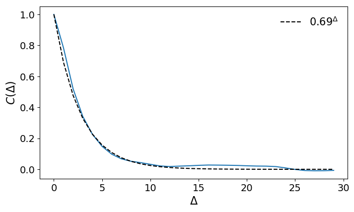
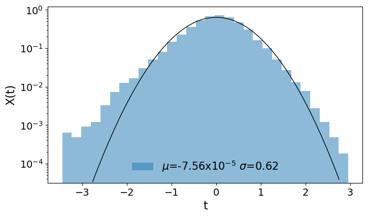
- The linear scaling and convergence to the Gaussian distribution holds in the long t limit if the random variables are correlated (not independent) with a finite correlation time \[\tau = \sum_{t=1}^\infty C(t) < \infty.\]
- This can be seen by looking at the coarse grained time series with uncorrelated elements
Beyond the central limit theorem
Processes with increments x that
- do not have a finite variance (extreme events)
- are not identically distributed (changes over time)
- are not independent - event in the long time limit (in a later lecture)
Levy-stable Distributions
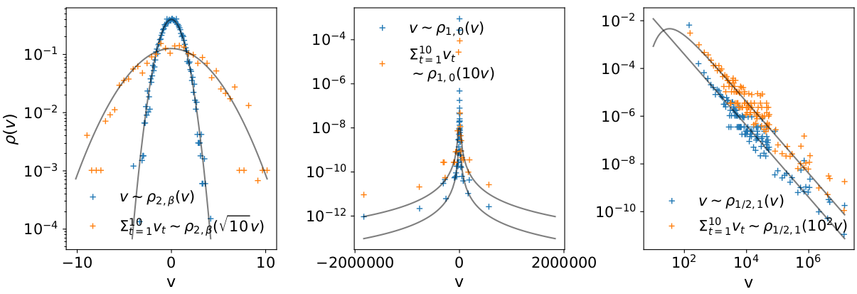 \[ \mathcal{F}[\rho_{\gamma,\beta}(x,\mu,\sigma)]=\rho_{\gamma,\beta}(k,\mu,\sigma) =\exp\left[ i\mu k - \sigma^\gamma |k|^\gamma \left( 1 - i\beta \frac{k}{|k|}w(k,\gamma)\right)\right] \]
\[ \rho_{\gamma,\beta}\left(\frac{\sum_{n=1}^t v(n)}{t^{1/\gamma}}\right)=\rho_{\gamma,\beta}\left(\frac{x(t)}{t^{1/\gamma}}\right) \]
\[ \mathcal{F}[\rho_{\gamma,\beta}(x,\mu,\sigma)]=\rho_{\gamma,\beta}(k,\mu,\sigma) =\exp\left[ i\mu k - \sigma^\gamma |k|^\gamma \left( 1 - i\beta \frac{k}{|k|}w(k,\gamma)\right)\right] \]
\[ \rho_{\gamma,\beta}\left(\frac{\sum_{n=1}^t v(n)}{t^{1/\gamma}}\right)=\rho_{\gamma,\beta}\left(\frac{x(t)}{t^{1/\gamma}}\right) \]
The Noah-Effect
(Mandelbrot and Wallis) \[ \rho(x(t)) = t^L \rho\left(x(t)/t^L\right) \] \[ y(t)=\sum_{s=1}^t x(s), \; \mbox{ with } \; \langle x(s)x(s+\Delta)\rangle=\delta(\Delta), \; \mbox{ and } \; \lim_{x\rightarrow\infty}\rho(|x|)\propto |x|^{-3+2L}. \]- Power law tails lead to anomalous scaling (non-linear) \[ \langle y^2(t) \rangle \propto t^{2L}\]
- Slower decay in tails of the distribution has no effect on the MSD and the density approaches a Gaussian
Non-stationary Processes
- Idealized case: Increment variance grows or decays with power law over time (Scaled Brownian Motion) \[ x_t=t^{M-1/2}\xi_t \;\; \Rightarrow \;\; y(t)=\sum_{s=1}^t x(s) = t^{M} \sum_{s=1}^t \xi_t/\sqrt{t} \]
- Power law growth/ decay lead to anomalous scaling \[ \langle x^2(t) \rangle \propto t^{2M} \]
Non-stationary increments: What is shape of distribution and MSD scaling?
| variance grows/decays | variance random/periodic | |
|---|---|---|
| Gaussian increments | Gaussian/anomalous | Gaussian/normal |
| Non-Gaussian increments | Non-Gaussian/anomalous | Non-Gaussian/normal |
Air Pressure: Non-stationarity
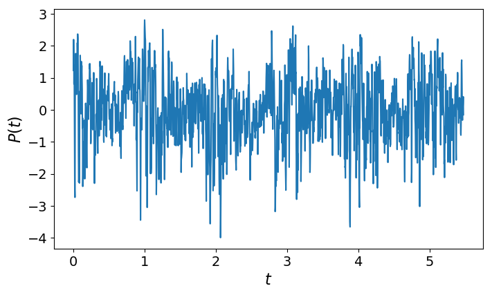
- Air pressure data from Potsdam
- Density is Non-Gaussian
- Trajectory shows: Variance changes with the Seasons
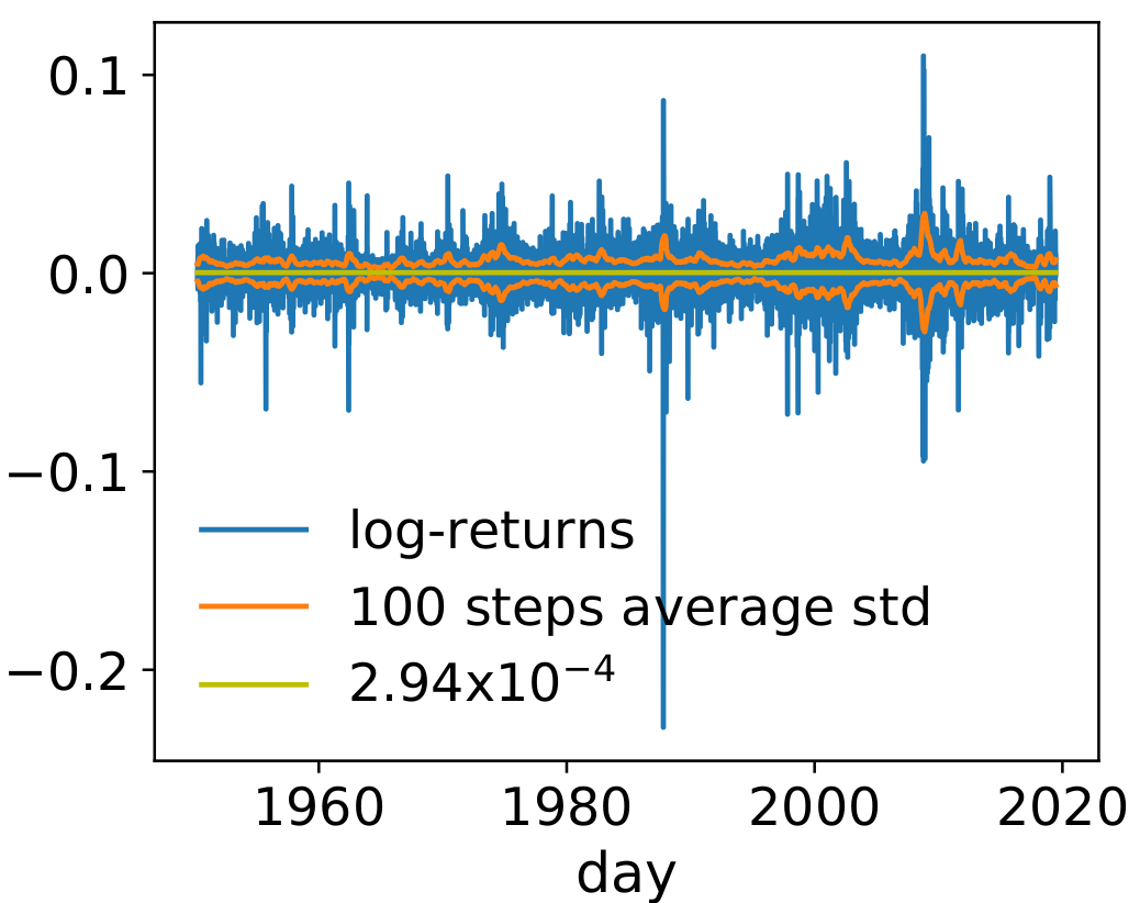
Correlated Volatility
- Look at S & P 500 index
- Financial assets are characterized by log-return
- Variance (volatility) is not constant, but correlated
- GARCH(1,1) Model \[ x_t = \sigma_t\xi_t \] \[ \sigma_t^2 = c + ax_{t-1}^2 + b \sigma_{t-1}^2 \]
Exterimental Observation: Non-Gausian with normal scaling of MSD
Experimental setup for non-Gaussian diffusion with linear scaling of MSD (see Pastore et al. 2022)Unicellular Dictyostelium discoideum: Anomalous scaling and non-Gaussian
Non-Gaussian diffusion and anomalous scaling in the diffusion of amoeboid cells (see Cherstvy et al. 2018)Ergodicity
Remember: a requirement for ergodicity is, that the dynamics is measure preserving
- Non-stationary increments and increments with diverging variance both lead to linear scaling in the time-averaged MSD, while the ensemble averaged MSD depends on the exact definition of the dynamics
Telomeres Diffusion: Non-ergodicity
In the diffusion of Telomeres, the time average of the MSD exhibits a different scaling from the ensemble average (see Bronstein et al. 2009)Random Events
Examples:
- Radioactive decay
- Volcanic erruptions
A random event might occur at any moment in time with probability lambda
- What is the probability distribution of the event happening at time t \[ p(t=0) = \lambda \] \[ p(t=1) = (1-\lambda) \lambda \] \[ p(t) = (1-\lambda)^t\lambda \approx e^{-\lambda t} \lambda \; \; \mbox{with} \; \lambda=\frac{1}{\tau} \]
The Poisson Prozess
A process with interevent times
\[W(\tau) = {\lambda} \exp(-\lambda \tau) \]Generally, the probability of N events in the time interval t is given by the binomial distribution
\[ \Lambda = t\lambda \] \[ \frac{t!}{N!(t-N)!} \lambda^N(1-\lambda)^{t-N} \approx \frac{\sqrt{2\pi t}(t/e)^t}{\sqrt{2\pi(t-N)}((t-N)/e)^{t-N}}\lambda^N (1-\lambda)^{t-N} \] \[ \approx \frac{t^t \lambda^N(1-\lambda)^{t-N}e^{-N}}{(t-N)^{t-N} N!} \approx \frac{t^t (\Lambda/t)^N(1-\Lambda/t)^{t-N}e^{-N}}{t^{t-N}(1-N/t)^{t-N} N!} \approx \frac{\Lambda^N (1-\Lambda/t)^{t} e^{-N}}{(1-N/t)^{t} N!} \approx \frac{\Lambda^N e^{-\Lambda}}{N!} \]Continuous time random walks
- There is a general class of processes with interevent duration distribution W(t)
- In addition, we can define a random walk y(t), where the time between two steps is defined by W(t)
- The distribution of jumplengths can then be drown from a second probability distribution
- Or both distribution can be coupled, i.e. the joint probability distribution reads \[ \Psi(\chi,\tau) = W(\tau) \frac{1}{2} [ \delta(\chi-f(\tau)) + \delta(\chi+f(\tau)) ] \]
Levy walks
Instead of jumps after each waiting period, the velocity can also be constant or grow/decay during the waiting period
More on these processes later, when we talk about Long Range Correlations
Aging
What happens if the distribution of waiting times W(t) has no finite mean?
\[ W(\tau) = \frac{u^\alpha}{\tau^{1+\alpha}} \;\; \mbox{ with } \;\; 1 > \alpha > 0 \]- The probability of an observation x(t) happening during a waiting period increases over time
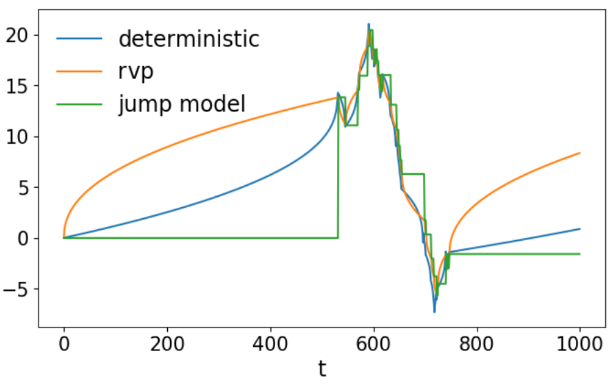
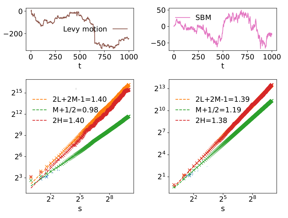
Anomalous scaling: How to distinguish extreme events and non-stationarity
[Chen et al. 2017]Look at first and second moments of the increments
- Non-stationary increments: \[ \langle \sum_t |x_t| \rangle = \sum_t t^{M-1/2} \langle |\xi_t| \rangle = t^{M+1/2} \langle |\xi_t| \rangle \] \[ \langle \sum_t x_t^2 \rangle = \sum_t t^{2M-1} \langle \xi_t^2 \rangle = t^{2M} \langle \xi_t^2 \rangle \]
- Infinit variance: \[ \rho(|x|) \rightarrow |x|^{-3+2L} \mbox{ for } |x|\rightarrow\infty \mbox{ with } 1>L>1/2 \] \[ \langle |x_t| \rangle \mbox{integrable, constant} \] \[ \langle x_t^2 \rangle \mbox{not integrable} \Rightarrow \mbox{grows with time} \]
Aging systems: L=3/4-M/2, both moments have the same time-dependent
Anomalous scaling: Example
Time-Reversal Symmetry
Gaussian Prozesses are time-reversal processes
When is time-reversal symmetry violated