The AR(1) process as a low pass filter

• Treat the noise term as your signal
• The AR(1) process smoothens this signal
• In other words, it increses autocorrelations for short times

Moving Averages

• Sliding window average
• Similar effect to AR(1) process

'Online Learning'

• We have a series of measurements for a variable Z
• Each measurement has some uncertainty
• What is the best estimation after each new measurement

• Much less storage is neccessary, compared to calculating the mean after each step

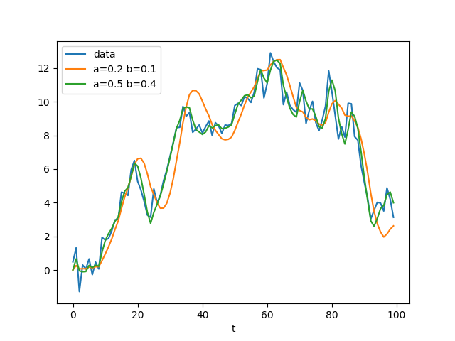
Alpha-Beta-Filter

What if we want to estimate a parameter, that is not constant

Update

Predict

Alpha-Beta-Filter: Example

Tracking a random walker

Kalman Filter weights

Similar to the alpha-beta-filter, the Kalman filter makes estimates based on the previous estimate and the latest measurement z

Treating x as a stochastic variable, we can look at the variance

Now we minimize p

Kalman Filter 1D constant state

Update

Predict

• Assumption: Gaussian errors, so distribution is given by mean and variance
• estimations for the variance p are independent of the measurements
• the weight is called Kalman gain \[ K_t = \frac{p_{t-1}}{p_{t-1}+r_t} , \; \; \mbox{ with } \; \; 1>K_t>0 \]

Bayes Theorem

• Prior P(M)
• Posterior P(M|D)
• Likelihood P(D|M)
• Evidence P(D)

Simple example

A test that can be positive p or negative n, is used by a person that can be infected i or healthy h

Second test with prior P(i)=0.12

Bayesian Filter

In our case, Bayes' rule defines the update step in general as \[ P(x_t|z_{1...t}) = \frac{P(z_t|x_t) P(x_t|z_{1...t-1})}{P(z_t|z_{1...t-1})} = \frac{P(z_t|x_t) P(x_t|z_{1...t-1})}{\int P(z_t|x_t) P(x_t|z_{1...t-1})\mathrm{d}x_t} \]

• For Gaussian propability distributions, we only need the mean and the variance, to know the full distribution
• The Kalman filter is the solution for linear Gaussian systems

Find the derivation at https://people.bordeaux.inria.fr/pierre.delmoral/chen_bayesian.pdf

Linear Systems (The Kalman Filter)

Hidden Markov model

\[ x_{t} = F x_{t-1} + q_{t-1}\] \[ z_t = Hx_t +r_t \] Where q is Gaussian white noise with variance Q, r is Gaussian white noise with variance R, x is a vector, and A and H are matrices

Accordingly, the algorithm is update: \[ K_t = \frac{p_{t|t-1} H^T}{ Hp_{t|t-1} H^T + r_t } \] \[ x_{t|t} = x_{t|t-1} + K_t ( z_t-Hx_{t|t-1} ) \;\;\;\; p_{t|t} = (\mathbb{1}-K_t H) p_{t|t-1} (\mathbb{1} - K_t H)^T + K_t r_t K_t^T \] and prediction: \[ x_{t+1|t} = F x_{t|t} \;\;\;\;\; p_{t+1|t} = F p_{t|t} F^T + q_t \]

Find a slower introduction at www.kalmanfilter.net

Extended Kalman Filter

• If F and H are non-linear, we can use a linearized version

where the derivatives is given by the Jacobian matrices

• Leads to adjustment in the Kalman filter

Monte Carlo Approaches

• Recall the definition of the ensemble average \[ \langle f(x) \rangle = \int f(x)\rho(x)\;\mathrm{d}x \]
• In practice (in the exercise) this was measured by simulating M realizations (different initial conditions or process noise) of x_t, so the ensemble \[x_t^{(m)}\] represents the distribution at time t \[\rho(x_t)\]
• In the case of discrete states the probabilities can be easily identified as weights of the states \[ \sum_{i} f(x_i)P(x=x_i) = \frac{1}{M} \sum_m f(x^{(m)}) \]

Ensemble Kalman filter

The update step with NxN matrices in the Kalman filter is computationally costly. The ensemble Kalman filter approximates some quantities and reduces the dimensions to Nxn with N>n

• Create an ensemble \[ X = [x^{(1)},...,x^{(n)}] \]
• Create a corresponding ensemble of the data, by adding a random vector to each copy of the measurement vector \[ Z = [z^{(1)},...,z^{(n)}] \]
• Then we can calculate \[ X_{t|t} = X_{t|t-1} + K(Z-HX_{t|t-1}) \] with \[ K_t=Q_tH^T (HQ_tH^T + R_t)^{-1} \] where the covariance Q can now be computed from the ensemble X_t

Such an approximation is called a Monte-Carlo approximation

Back to Bayes' Theorem

Optimizing the parameters theta

The task of parameter estimation

Calculating the Likelihood

with

The update and prediction steps are performed with some Bayesian filter (e.g. the Kalman filter)

From the likelihood to the optimal parameter

Numerically more stable: the energy function

Solve by

So the optimal parameter is given by

• Expectation values can then be calculated from the posterior

Example: the SEIR model

With N=S+E+I+R constant

No birth and death: m->0

Reproduction number

Some parameters can be estimated, i.e. g=1/3 per day, a=1/5.2 per day

Task: Find contact parameter b

The probabilistic SEIR model

With X=(S,E,I,R); Observable state: Y=I+R; corresponding measurements z

Kahlman filter: \[ X_{t|t} = X_{t|t-1} - \frac{1}{2} K_{t} (Y_{t|t-1} + \langle Y _{t|t-1} \rangle - 2 ) \] Kahlman gain \[ K_t = \frac{\langle (X_{t|t-1}-\langle X_{t|t-1}\rangle)[(I_{t|t-1}-\langle I_{t|t-1}\rangle)+(R_{t|t-1}-\langle R_{t|t-1}\rangle)] \rangle}{\langle (I-\langle I \rangle)^2 \rangle + 2\langle (R-\langle R\rangle)(I-\langle I\rangle ) \rangle + \langle (I-\langle I \rangle)^2 \rangle + r} \] estimated observation error r=10

SEIR Parameter Estimation

Approximate Log-Likelihood as \[ L(t,b) = \frac{1}{2} \frac{|(\langle I \rangle-z_I)+(\langle R \rangle-z_R)|^2}{\langle (I-\langle I \rangle)^2 \rangle + 2\langle (R-\langle R \rangle)(I-\langle I\rangle) \rangle + \langle (I-\langle I \rangle)^2 \rangle + r} \] \[\;\;\;\;\;\;\;\;\;\;\;\;\;\;\;\;\;\; + \frac{1}{2} \log(\langle (I-\langle I \rangle)^2 \rangle + 2\langle (R-\langle R\rangle)(R-\langle R\rangle ) \rangle + \langle (I-\langle I \rangle)^2 \rangle + r), \]

Assuming a Gaussian Likelihood function \[ -\log( \frac{1}{\sigma_Y}e^{-\Delta Y/(2\sigma_Y^2)} ) = -\frac{1}{2}\log(\sigma_Y^2) - \frac{\Delta Y}{2\sigma_Y^2} \] Obtain b by minimizing \[ b^* = argmin_b \sum_t L(t,b) \]

Sequential data assimilation of the SEIR model for COVID-19

Markov Chain Monte Carlo

If we do not assume Gaussian distributions, the observables like mean and variance have to be calculated from the posterior. Markov Chain Monte Carlo is a method to approximate

Require:

• Ergodicity
• Detailed Balance
• Markov property

Construct a series x_t of length T that has the probability distribution \[\rho(x)\], then \[ \langle f(x) \rangle = \frac{1}{T} \sum_t f(x_t) \]

The Metropolis-Hastings Algorithm

Detailed Balance

Defining the proposal distribution Q and the acceptance distribution T \[ p(\Theta_{t+1}|\Theta_t)= Q(\Theta_{t+1}|\Theta_t) T(\Theta_{t+1}|\Theta_t) \]

So \[\frac{T(\Theta_{t+1}|\Theta_t)}{\Theta_{t}|\Theta_{t+1}} = \frac{p(\Theta_{t+1})}{p(\Theta_t)} \frac{Q(\Theta_{t}|\Theta_{t+1})}{Q(\Theta_{t+1}|\Theta_t)}\]

This is fulfilled by \[ T(\Theta_{t+1}|\Theta_t) = \min\left[1, \frac{p(\Theta_{t+1})}{p(\Theta_t)} \frac{Q(\Theta_{t}|\Theta_{t+1})}{Q(\Theta_{t+1}|\Theta_t)} \right] \]

At each point in time, draw sample from Q and compute the corresponding transition probability T. Then generate a random number u between 0 and 1, If u is smaller than T, accept the move and otherwise reject it

Effective Sample Size

• Rejected moves lead to autocorrelations and, therefore, reduced effective sample sizes
• The first iterations ofthe markov chan can not be used, as they depend on the initial value of the series, which might have a very low probability itself