Timescales in simple models

• Exponential dacay of autocorrelations: one characteristic timescale
• Power-law decay of autocorrelations: no characteristic timescale
• Oscillations: one characteristic timescale

Cycles

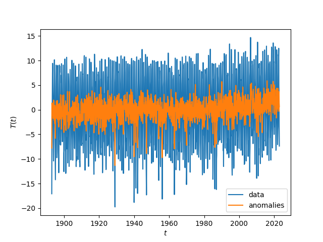
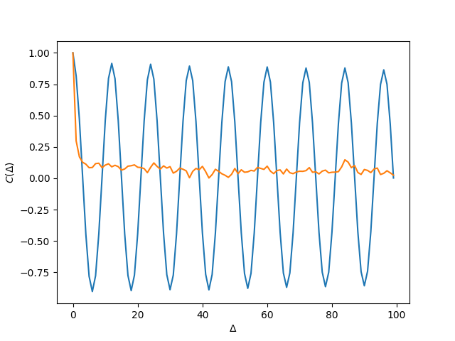
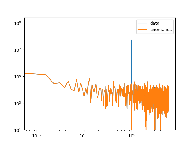
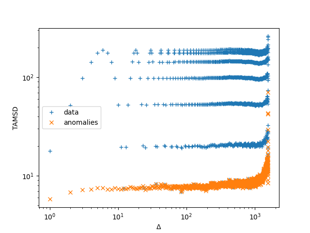
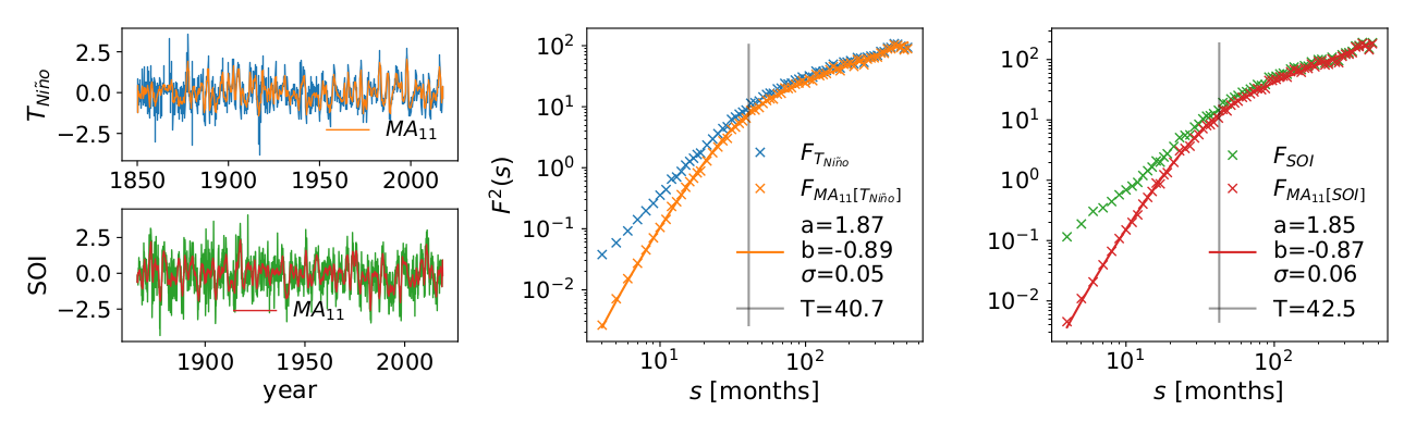
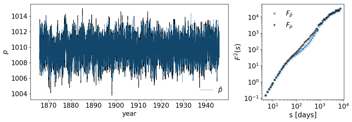
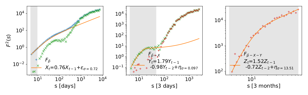
Various measures of autocorrelations of Temperature data from Potsdam. Effect of removing the deasonal cycle by subtracting mean values of each calendar day (Temperature anomalies).

Noisy oscillations

Noisy oscillations contain two timescales: the oscillatory mode and the decay auf autocorrelations

Underdamped harmonic oscillator \[ \ddot{x}(t) + \zeta \omega_0 \dot{x}(t) + \omega_0^2 x^2(t) = \xi(t) \] \[ [ x_{t+1} - 2x_t + x_{t-1} ] + \zeta\omega_0 [x_{t+1}-x_t] + \omega_0^2 x_t^2 = \xi_t \] \[ x_{t+1} = \frac{2+\zeta\omega_0 - \omega_0^2 }{1+\zeta\omega_0} x_t - \frac{1}{1+\zeta\omega_0} x_{t-1} = \xi_t \]

The autoregressive model of order two AR(2) \[ x_{t+1} = a x_t + b x_{t-1} + \xi_t \] \[ \mbox{with} \;\; b>-1 \;\;\;\; \mbox{stationary if} \;\; 1-|a|>b \;\;\;\; \mbox{oscillates if} \;\; -a^2/4>b \]

Autocorralation function of noisy oscillation has the form \[ C(\Delta) = e^{-\Delta/\tau} \cos(\omega \Delta + \phi) \]

Example: El Nino Southern Oscillation

Superpositions

A signal composed of two independent components y,z \[ x_t = y_t + z_t \]

• The autocovariance function \[ \langle x_{t_1}x_{t_2} \rangle = \langle (y_{t_1}+z_{t_1})(y_{t_2}+z_{t_2}) \rangle = \langle y_{t_1}y_{t_2}+y_{t_1}z_{t_2}+z_{t_1}y_{t_2}+z_{t_1}z_{t_2} \rangle = \langle y_{t_1}y_{t_2} \rangle + \langle z_{t_1}z_{t_2} \rangle \] is the superposition of the autocovariance functions of both components
• The same holds for the MSD or the variance \[ \langle x^2(t) \rangle = \langle y^2(t) \rangle + \langle z^2(t) \rangle \;\;\; \mbox{or} \;\;\; \langle (x(t)-\mu_x)^2 \rangle = \langle (y(t)-\mu_y)^2 \rangle + \langle (z(t)-\mu_z)^2 \rangle \]
• So, the autocorrelation function is \[ C_{xx}(\Delta) = \frac{ \langle y_{t_1}y_{t_2} \rangle + \langle z_{t_1}z_{t_2} \rangle }{ \sigma_y^2 + \sigma_z^2 } = \frac{ \sigma_y^2 C_{yy}(\Delta) + \sigma_z^2 C_{zz}(\Delta) }{ \sigma_y^2 + \sigma_z^2 } \]

• The superposition principle also holds for the TAMSD \[ \overline{{\delta_x}_\Delta^2} = \frac{1}{t-\Delta} \sum_{n=1}^{t-\Delta} (y_{n+\Delta}+z_{n+\Delta}-y_{n}-z_{n})^2\;\;\;\;\;\;\;\;\;\;\;\;\;\;\;\;\;\;\;\;\;\;\;\;\;\;\;\;\;\;\;\;\;\;\;\;\;\;\;\;\;\;\;\;\;\;\;\;\;\;\;\; \] \[ = \frac{1}{t-\Delta} \sum_{n=1}^{t-\Delta} (y_{n+\Delta}-y_n)^2+2(y_{n+\Delta}-y_n)(z_{n+\Delta}-z_n)+(z_{n+\Delta}-z_{n})^2 \] \[ = \frac{1}{t-\Delta} \sum_{n=1}^{t-\Delta} (y_{n+\Delta}-y_n)^2+(z_{n+\Delta}-z_{n})^2 = \overline{{\delta_y}_\Delta^2} + \overline{{\delta_z}_\Delta^2} \;\;\;\;\;\;\;\;\;\;\;\;\;\;\;\;\;\;\;\;\;\;\; \]
• ... and the power spectrum \[ X(\nu) = \int \mathrm{d}t\; [y(t)+z(t)] e^{-\frac{2\pi i}{N}t\nu} = Y(\nu) + Z(\nu) \] \[ |X(\nu)|^2 = |Y(\nu) + Z(\nu)|^2 = |Y(\nu)|^2 + |Z(\nu)|^2 \]

Measurement uncertainty and noise

No measured value is accurate - there is always some uncertainty with every value; we have to distinguish systematic errors and random errors

• Systematic errors have to be considered in models in different ways
• Example: Dynamic error for tracking particles \[ X(t)=\frac{1}{s}\int_0^sx(t-s_1)ds_1. \]
• Uncertainty usually comes in the form of uncorrelated additive noise \[ y(t)=x(t)+\xi(t) \]

Random error - effect on statistics

• Superpostition of a white noise term and the actual signal \[ y(t)=x(t)+\xi(t) \;\;\; \mbox{with} \;\;\; \langle \xi(t)\xi(t+\Delta) \rangle = \sigma_\xi^2 \delta(\Delta) \;\;\; \mbox{and} \;\;\; \langle x(t)x(t+\Delta) \rangle = \sigma_x^2 C_{xx}(\Delta) \]
• The correlation time for a model with \[C_{xx}=e^{-\Delta/\tau}\] decreases when superimposed with white noise \[ C_{yy}(\Delta) = \int_{\epsilon\rightarrow 0}^\infty \frac{\sigma_\xi^2\delta(\Delta)+\sigma_x^2e^{-\Delta/\tau}}{\sigma_\xi^2+\sigma_x^2} \mathrm{d}\Delta = \tau \frac{\sigma_x^2}{\sigma_x^2+\sigma_\xi^2} \]
• TAMSD \[ \langle \overline{\delta^2(\Delta)} \rangle = 2\sigma_x^2 (1-e^{-\Delta/\tau})+ 2\sigma_\xi^2 \]

What is a trend?

What is a trend? There are different interpretations

• Climate (global warming)
• Finance (inflation)
• ...

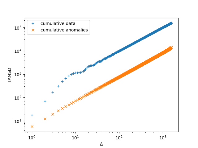
Example of Temperatures station data at Indonesia

Example of Temperatures station data at Indonesia

Summary

• Complex time series can have several characteristic time scales
• Time scales can be approximated by relaxations (overdamped motion) and noisy oscillations (underdamped motion)
• Measurement noise typically imvolves white noise, so it fluctuates on the shortest time scale
• The largest time scale in some systems is treated as a trend; it can be a 'real' (infinite) trend or just a very long timescale compared to the length of the time series