7. Spectra
The Autocorrelation Function and the MSD
As shown in previous chapters, the MSD is directly connected to the velocity autocovariance
\[ \langle (x(t-t_0)-x(t_0))^2 \rangle = 2 \int_{0}^{t} \mathrm{d}t_1 \int_{t_1}^t \mathrm{d}t_2 \langle \dot{x}(t_0+t_1) \dot{x}(t_0+t_2) \rangle = 2 \int_{0}^{t} \mathrm{d}t_1 \int_{t_1}^t \mathrm{d}t_2 C(t_2-t_1) \sigma^2(t_0+t_1) \]The ensemble-averaged MSD with a fixed initial time, e.g. x(t0)=0, depends on non-stationarity
By calculating the time average, the integral over the total time eliminates this time dependence
\[ \langle \delta^2(\Delta) \rangle = \frac{2}{t-\Delta} \int_0^{t-\Delta} \mathrm{d}t_0 \int_{0}^{\Delta} \mathrm{d}t_1 \int_{t_1}^\Delta \mathrm{d}t_2 \langle \dot{x}(t_0+t_1) \dot{x}(t_0+t_2) \rangle \] \[\;\;\;\;\;\;\;\;\;\;\; = \frac{2}{t-\Delta} \int_0^{t-\Delta} \mathrm{d}t_0 \int_{0}^{\Delta} \mathrm{d}t_1 \int_{t_1}^\Delta \mathrm{d}t_2 C(t_2-t_1) \sigma^2(t_0+t_1) \]Example: power-laws: Using the exponents defined in the previous chapters J, M, and L, it can be shown \[ \langle x^2(t) \rangle \sim t^{2J+2M+2L-1} \;\;\;\;\;\; \langle \delta^2(\Delta) \rangle \sim \Delta^{2J} \]
Sinusoidal signals
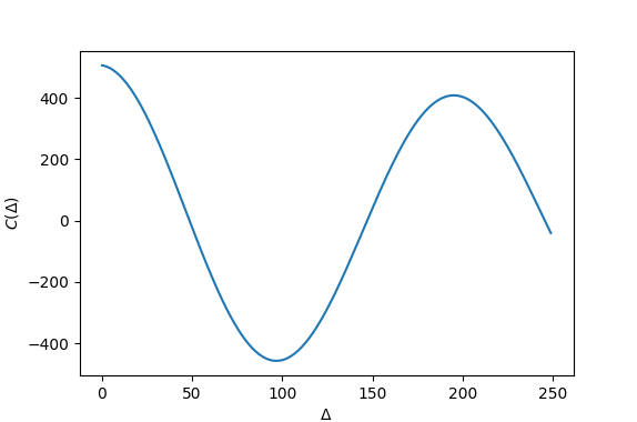
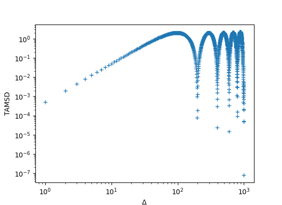
Autocorrelation function and time-averaged MSD both oscillate - no nice measures for the frequency of oscillation
Problems of the autocorrelation function
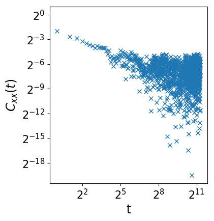 Very noisy for long lag times
 Timescales mix
The autocorrelation function is useful for theoretical considerations and interpretations, but not always suitable for data analysis
The Power Spectrum
The Power Spectrum is the square of the Fourier transform of the signal; it therefore nicely resolves oscillations
\[ X(\nu) = \int \mathrm{d}t\; x(t) e^{-\frac{2\pi i}{N}t\nu} \] \[ x(t) = \int \mathrm{d}\nu\; X(\nu) e^{\frac{2\pi i}{N}t\nu} \] \[ |X(\nu)|^2 = X(\nu)\overline{X}(\nu) = \int \mathrm{d}t^\prime \int \mathrm{d}t\; x(t) x(t^\prime) e^{-\frac{2\pi i}{N}(t-t^\prime)\nu} \]The Wiener-Khinchin Theorem
The connection between the autocorrelation function and the power spectral density can be calculated straightforwardly. The autocorrelation function is \[C(\Delta)=\int_{-\infty}^\infty \overline{x}(t) x(t+\Delta) \mathrm{d}t\] The Fourier transform of X and its complex conjugate is \[ x(t)=\int_{-\infty}^\infty X(\nu) e^{-2\pi i \nu t} \mathrm{d}\nu \mbox{ } \mbox{ } \mbox{ and } \mbox{ } \mbox{ } \overline{x}(t)=\int_{-\infty}^\infty \overline{X}(\nu) e^{2\pi i \nu t} \mathrm{d}\nu\] If we now plug in the Fourier transform into the definition of the autocorrelation function, we get the Fourier transform of the power spectrum \[C(\Delta) = \int_{-\infty}^\infty \left[ \int_{-\infty}^\infty X(\nu) e^{-2\pi i \nu (t+\Delta)} \mathrm{d}\nu \right] \left[ \int_{-\infty}^\infty \overline{X}({\nu'}) e^{2\pi i \nu' t} \mathrm{d}\nu' \right] \mathrm{d}t \;\;\;\;\;\;\;\;\;\;\;\;\;\;\;\;\;\;\;\;\;\;\;\;\;\;\;\;\;\;\;\;\;\;\;\;\;\;\;\;\;\;\;\;\;\;\;\;\;\;\;\;\;\;\;\;\;\;\;\;\;\;\;\;\] \[\mbox{ } = \int_{-\infty}^\infty \int_{-\infty}^\infty \int_{-\infty}^\infty \overline{X}(\nu) X({\nu'}) e^{-2\pi i (\nu'-\nu) t} e^{-2\pi i \nu \Delta} \mathrm{d}t \mathrm{d}\nu \mathrm{d}\nu = \int_{-\infty}^\infty \int_{-\infty}^\infty \overline{X}(\nu) X({\nu'}) \delta(\nu'-\nu) e^{-2\pi i \nu' \Delta} \mathrm{d}\nu \mathrm{d}\nu^\prime \] \[= \int_{-\infty}^\infty \overline{X}(\nu) X({\nu}) e^{-2\pi i \nu \Delta}\mathrm{d}\nu = \int_{-\infty}^\infty |X({\nu})|^2 e^{-2\pi i \nu \Delta}\mathrm{d}\nu = \mathcal{F}_\nu \left[ |X(\nu) |^2 \right](\Delta) \;\;\;\;\;\;\;\;\;\;\;\;\;\;\;\;\;\;\;\;\;\;\;\;\;\;\;\;\;\;\;\;\;\;\;\;\;\;\; \]
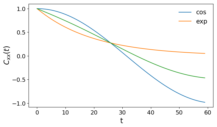
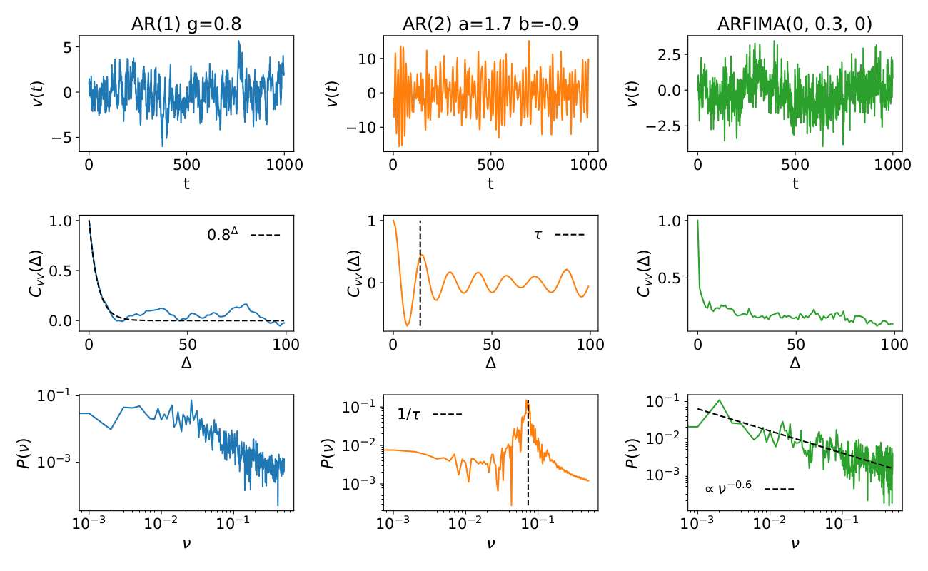
Examples
Autocorrelation function and power spectrum for
- a signal with exponentially decaying autocorrelations
- a signal with oscillatory behavior
- a signal with power-law decay of correlations
Wavelets
\[ d_{j,k} = \int_{-\infty}^\infty x(t) \Psi_{j,k}^* \mathrm{d}t \]Where the wavelet Psi is a function
- which is localized in the time-domain
- the integral over the function is zero
- wavelets with different j are orthogonal to each other


 https://upload.wikimedia.org/wikipedia/commons/a/a0/Haar_wavelet.svg
https://upload.wikimedia.org/wikipedia/commons/1/19/Wavelet_-_Morlet.svg
https://upload.wikimedia.org/wikipedia/commons/0/01/Wavelet_-_Mex_Hat.png
https://upload.wikimedia.org/wikipedia/commons/a/a0/Haar_wavelet.svg
https://upload.wikimedia.org/wikipedia/commons/1/19/Wavelet_-_Morlet.svg
https://upload.wikimedia.org/wikipedia/commons/0/01/Wavelet_-_Mex_Hat.png
The Wavelet Transform
\[ d_{j,k} = \int_{-\infty}^\infty x(t) \Psi_{j,k}^* \mathrm{d}t \] \[ \Psi_{j,k}(t) = \frac{1}{\sqrt{2^j}} \Psi(2^{-j}t-k) \] \[ x(t) = \frac{1}{C} \int_0^\infty \sum_{j=0}^\infty d_{j,k} \Psi_{j,k} \frac{\mathrm{d}j\;\mathrm{d}k}{2^j} \]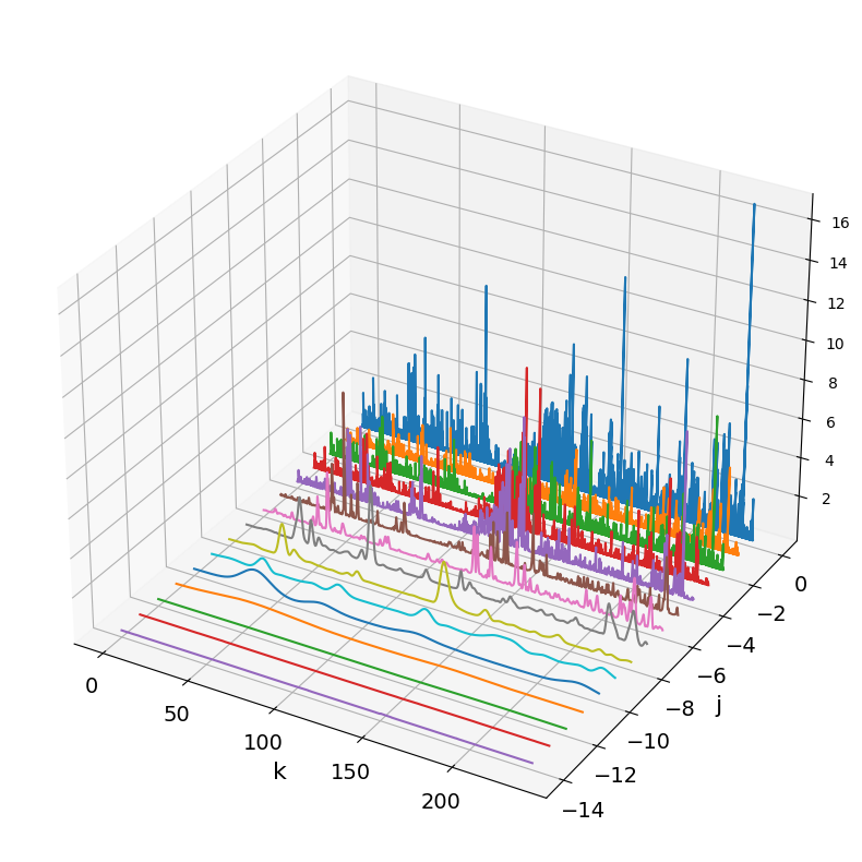 Wavelet transform of a the increments of a trajectory of a tracked animal
The parameter k can resolve non-stationarities in the signal
Averaging over the the k-parameter
\[ F_j = \frac{1}{K}\sum_{k=0}^K |d_{j,k}|^2 \]Is a scaling function similar to the time-averaged mean squared displacement (TAMSD)
The Poor Man's Wavelet and the TAMSD
\[ \Psi(t) = \delta(t) - \delta(t-\tau) \]satisfies the conditions of a wavelet
The wavelet transform with above expression yields \[ d_{j,k} = \int_{-\infty}^\infty x(t) \frac{1}{\sqrt{2^j}} (\delta(2^{-j}t-k) - \delta(2^{-j}t-k-\tau)) \mathrm{d}t \] \[ =\frac{1}{\sqrt{2^j}} [x(2^{j}k) - x(2^{j}(k+\tau))] \] The corresponding scaling function is \[ F_j = \frac{1}{2^jK}\sum_{k=0}^K [x(2^{j}k) - x(2^{j}(k+\tau))]^2 \] which is the same as the TAMSD
Smoothening via the Wavelet transform
The wavelet transform can be used as a filter
- Set all elements for small j to zero and back-transform to physical space: small timescales (noise) are removed
- Set all elements for large j to zero and back-transform to physical space: long timescales (trends) are removed
DFA to the Autocorrelation Function
Detrended fluctuation analysis [Peng et al. (1994)]:
where p is a polynomial of order q
DFA0 corresponds to the TA MSD with a specific averaging
Larger q lead to filtering out slow trends in the signal
DFA(1) with linear fits in each segment of length s
Summary
The following measures can express equivalent information as the autocorrelation function, however, they emphasis on different properties of the signal
- Autocorrelation function \[C(\Delta )=\frac{1}{T\sigma^2}\sum_{t=1}^{T} x(t)x(t+\Delta) \]
- Time average mean squared displacement \[\overline{\delta^2}(t,\Delta) = \frac{1}{t-\Delta} \sum_{t_0=0}^{t-\Delta} \left[ y(t_0+\Delta) - y(t_0)\right]^2 \]
- Detrended fluctuation analysis \[F_q^2(s)=\left\langle\frac{1}{s}\sum_{t=1}^{s} \Big(y(t+(n -1) s)-p_{n,s}^{(q)}(t)\Big)^2\right\rangle_n\]
- Power Spectral Density \[S(f)=|\mathcal{F}x(t)|^2\]
- Wavelet analysis
https://upload.wikimedia.org/wikipedia/commons/9/95/Continuous_wavelet_transform.gif