2. Autokorrelationen
What will the weather be like tomorrow?
Temperature T(t)=?
- Like today? T(t-1)
- Like the average of the last years on the same calendar day? Climatology C(t)
- Something in between?
Autoregressive Prozess of Order one AR(1)
\[ x_t = m(1-a) + a x_{t-1} + \xi_t \]- The parameter a is smaller than 1
- The expected value is between x(t-1) and the long time average (zero)
- The noise describes an uncertainty - so the real value of x(t) might as well be larger than x(t-1) or have the opposite sign
- m can be set to 0 by subtracting the mean value from the data
In the example of tomorrow's weather, we define the observable as \[x(t)=T(t)-C(t),\] where C(t) is the long time average on the specific calendar day
Variance of the AR(1) Process
The variance\[\sigma_x^2=\langle (x-m)^2 \rangle \]
of the AR(1) process with zero mean \[ x_t = a x_{t-1} + \xi_t \]
is the average of the squared process for large t
\[ \langle x_t^2 \rangle = \langle a^2 x_{t-1}^2 \rangle + 2 \langle a x_{t-1} \xi_t \rangle + \langle \xi_t^2 \rangle\] \[ \sigma_x^2 = a^2 \sigma_x^2 + 0 + \sigma_\xi^2 \] \[ \sigma_x^2 (1-a^2) = \sigma_\xi^2 \] \[ \sigma_x^2 = \frac{\sigma_\xi^2}{1-a^2} \]Relaxations
\[x_{t+1} = ax_{t} + \xi_t = a(ax_{t-1}+\xi_{t-1})+\xi_t\]Going forward more than one step, the expected value of x(t+s) goes to zero
\[x_{t+\Delta} = a^{\Delta+1} x_t + \xi_t^* \; \mbox{ with } \; \xi_t^*= \sum_{i=1}^{\Delta} a^{i-1}\xi_{t+i-1} \]The Autocorrelation Function
Autocovariance: \[ \langle x(t_1)x(t_2) \rangle \]
Autocorrelations: \[ C(t) = \frac{1}{\sigma^2} \langle x(t+\Delta)x(t) \rangle \]
Describes the expected dynamics of a noisy or chaotic process
It not only captures relaxations, but also oscillations and multiple timescales
The Autocorrelation Function of the AR(1) Prozess \[ \langle x_{t+\Delta} x_t \rangle = a \langle x_{t+\Delta-1} x_t \rangle = a^\Delta \langle x_t^2 \rangle = a^\Delta \sigma_x^2 \] \[C(\Delta)=a^\Delta\]
The Autocorrelation Time
The autocorrelation time is defined as \[\tau = \int_{0}^\infty C(t) \mathrm{d}t\]
We see that for AR(1) \[\tau = \int_{0}^\infty a^t \mathrm{d}t = \int_{0}^\infty e^{-\log(a)t} \mathrm{d}t = -1/\log(a).\] We can find a corresponding time-continuous process with the same autocorrelation function \[ \dot x(t) = -x(t)/\tau + \xi(t)\]
The Overdamped Harmonic Oscillator
\[\dot x(t) = -\frac{m\omega^2}{\eta} x(t) + \xi(t)\]This is solved by
\[x(t) = x(0)e^{-{m\omega^2}t/{\eta}} + \int_0^t \xi(s) e^{{m\omega^2}(t-s)/{\eta}} \mathrm{d}s \stackrel{x(0)=0}{=} \int_0^t \xi(s) e^{{m\omega^2}(t-s)/{\eta}} \mathrm{d}s \]Accordingly, the autocovariance is
\[\langle x(t) x(t+\Delta) \rangle = \int_0^t \mathrm{d}t_1 \int_0^{t+\Delta} \mathrm{d}t_2 \langle\xi(t_1) \xi(t_2)\rangle e^{{m\omega^2}(t-t_1)/{\eta}} e^{{m\omega^2}(t+\Delta-t_2)/{\eta}} = \sigma_\xi^2 \frac{\eta}{m\omega^2} \left( e^{-{m\omega^2}\Delta/{\eta}} - e^{-2{m\omega^2}t/{\eta}} \right) \] \[C(\Delta)= e^{-\Delta/{\tau}} \mbox{ , with } \;\;\; \tau= \frac{\eta}{m\omega^2} \mbox{ , and } \;\;\; \sigma_x^2 = \tau\sigma_\xi^2 \]Recall, for the discrete AR(1) process, we have \[C(\Delta)= e^{-\Delta/{\tau}} \mbox{ , with } \;\;\; \tau= -\frac{1}{\log(a)} \mbox{ , and } \;\;\; \sigma_x^2 = \sigma_\xi^2/(1-e^{-1/\tau}) \]
The Mean Squared Displacement
Starting from the \[ \langle x^2(t) \rangle = 2 e^{-2t/\tau} \int_{0}^{t} \mathrm{d}t_1 \int_{t_1}^t \mathrm{d}t_2 e^{t_1/\tau} e^{t_2/\tau} \langle \xi(t_1) \xi(t_2) \rangle \] \[ \mbox{ with } \; \langle \dot{x}(t_1) \dot{x}(t_2) \rangle = \sigma_\xi^2 e^{-|t_2-t_1|/\tau} \] \[ \langle x^2(t) \rangle = \sigma_\xi^2 \tau \left( 1 - e^{-2t/{\tau}} \right) \]
For short times t, the MSD scales linearly
\[ \langle x^2(t) \rangle = 2 \sigma_\xi^2 t \; \; \mbox{ with } \; \; D=\sigma_\xi^2 \]Air pressure
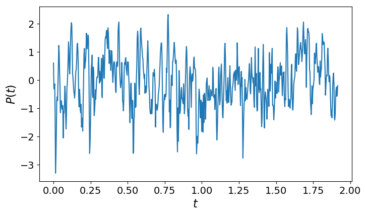
- Air pressure data from Moscow
- Data was corrected for seasonal effects
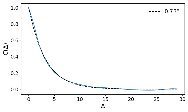
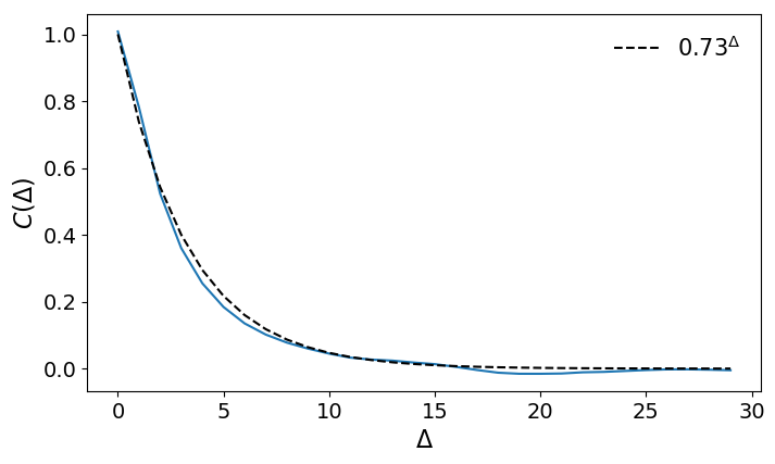
- Autocorrelation decays exponentially
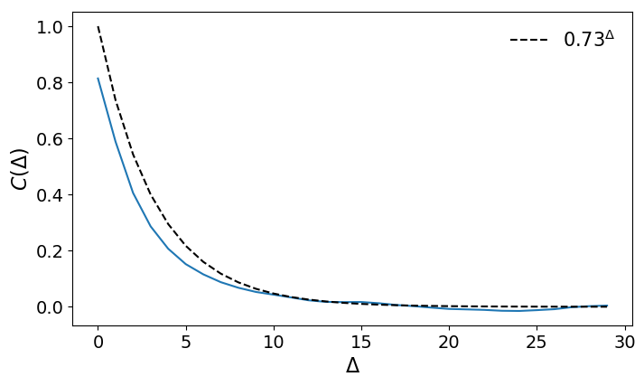
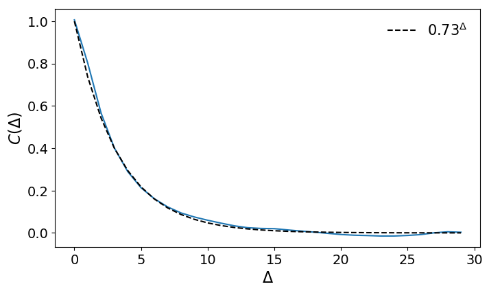
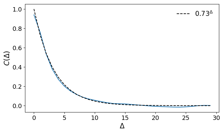
Time Resolution
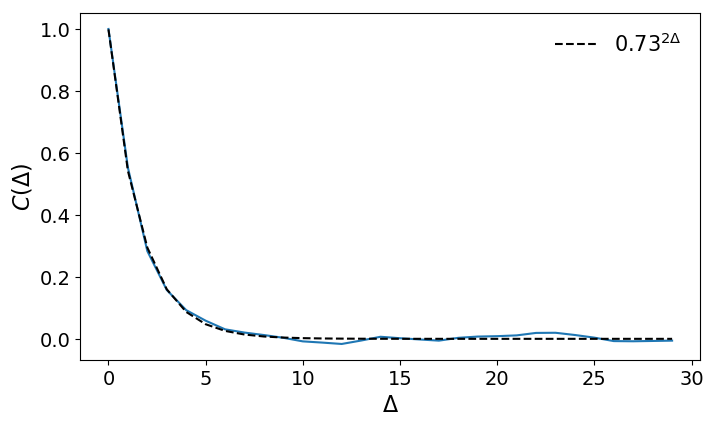
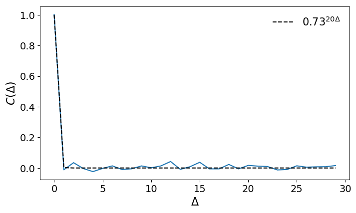
- Autocorrelation function of air pressure data with different time resolutions
Missing Values
Several ways to deal with it
- remove missing values [x1,x2,x4,x5]
- set missing values to mean value of the time series [x1,x2,m,x4,x5]
- set missing value to previous value [x1,x2,x2,x4,x5]
- set missing value to average of previous value and next value [x1,x2,(x2+x4)/2,x4,x5]
Accuracy of predictions decays over with time
- The model is not precise
- Unknown external influences
- Chaotic nature